Matching for Non Random Studies

Experimental designs such as A/B testing are a cornerstone of
statistical practice. By randomly assigning treatments to subjects, we
can test the effect of a test versus a control (as in a clinical trial
for a proposed new drug) or can determine which of several web page
layouts for a promotional offer receives the largest response. Designed,
controlled experiments are a common feature of much of scientific and
business research. THe internet is a natural platform from which to
launch tests on almost any topic, and the principles of randomization
are easily understood.

Unfortunately, not all data are collected in this manner. Observational
studies are still commonplace. In medicine, many published results rely
on the observation of patients as they receive care, as opposed to
participating in a planned study. On the internet, offers are often sent
to whitelists which are made up of non-randomly selected potential
customers. And in manufacturing, it may not always be possible to
control environmental variables such as temperature and humidity, or
operational characteristics such as traffic intensity.

The fact that treatments are not randomly assigned should not
necessarily mean that the data subsequently collected is of no use. In
this note we will discuss ways that researchers can adjust their
analysis to account for the way in which treatments were assigned or
observed. We begin with a study of men who were admitted to hospital
with suspicion of heart attack. There were 400 subjects, aged 40-70,
with mortality within 30 days as the outcome. The treatment of interest
in this case is whether a new therapy involving a test medication is
more effective than the standard therapy. The issue is that the new
therapy was not applied randomly, but rather that patient prognosis was
a partial determinant in which treatment was given.

The raw data shows a lower mortality rate for the treatment group:

This corresponds to an odds ratio of 0.687, suggesting lower overall
mortality for the treatment group (although a test for the hypothesis of
equal mortality rates does not reject at α = 0.05). The odds ratio in
this case is the ratio of the odds of death given the test relative to
the odds of death given the control; values less than 1 show a stronger
likelihood of survival for test subjects relative to control subjects.

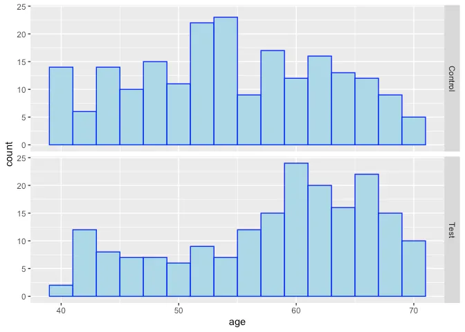
However, as suggested above, it does not appear that the treatment and
control are completely similar in terms of their covariates, as might be
expected in a fully randomized design – it appears that older subjects
and those with higher severity scores (a clinical rating of disease
severity) received the test at higher rates than the control:

Quantification of the treatment effect is at least partially confounded
with some of the underlying conditions that correlate with increased
expected mortality. So how to proceed? Regression (in this case,
logistic regression) is typically used to measure the effects of a
variable conditional on levels of the other variables, adjusting for
inequities in the distributions of the explanatory factors. Using a
logistic regression in this case, with a binary variable for treatment
(0 = Control, 1 = Test) and also linear variables for Age, Serverity,
and Risk Score (another prognostic assessment), we find that the odds
ratio for treatment vs control drops to 0.549, and is significantly less
than 1 at α = 0.05, with a 95% confidence interval of (0.31, 0.969).

However, this is an observational study, and to be useful, we need to
have more evidence that the effect of the test treatment can be measured
cleanly apart from the other variables AND from any (possibly
unintentional) selection biases that might arise due to the way
treatments were assigned to patients. That is, we need an unbiased
estimate of treatment effect, i.e., the effect of the test treatment
have if applied to the entire population of interest. To do this, we
need to introduce the concept of a counterfactual.

Propensity Scores and Other Matching Methods

In a perfect world, we would be able to measure the effect of both the
treatment and control on each subject. In most cases, including our
example on heart attacks, such a measurement is not available and not
possible. If we denote the response to the test treatment as
Y₁ and the response to the control treatment as
Y₀, we see that only one of these is observable — subjects
that get the treatment correspond to Y₁ and subjects that
get the control correspond to Y₀. For each case, the
unobservable outcome is called a counterfactual, a conceptual quantity
that does not exist. If we use Z to indicate which treatment was applied
(Z = 1 for test and Z = 0 for control), then the observation Y can
be expressed as the sum of an observation and an unobserved
counterfactual:

Y = ZY₁ + (1 − Z)Y₀

For each subject we are interested in Y₁ − Y₀,
the difference between the observation and the unobserved
counterfactual. When looking at the target population as whole, we are
likely interested in the average treatment effect:

Δ = E(Y₁ − Y₀)=E(Y₁)−E(Y₀)

where E denotes expectation or average. Unless the treatment
assignment is independent of the other factors, estimates for Δ might
be biased. Matching and other approaches known as propensity scores
are among the techniques that can be used to make the assignment of test
and control appear more random.

A propensity score is an estimate of the “probability” that a subject
gets assigned to test or control. If assignment is completely random,
then the propensity score is simply 0.50 for all subjects (assuming
equal sizes go into test and control). It can be shown that if all the
characteristics used to determine both Z (assignment to test or
control) and (Y₀, Y₁) are known (e.g., age,
severity), then partitioning on this set of confounders X will allow
us to develop an unbiased estimate of Δ.

One form of partitioning is straightforward matching of test and
control subjects together when they share the same values of all
confounders. Matching may be easy to do when there are only one or two
confounders, but rapidly gets harder and the number of potential
confounders increases. A more flexible approach is propensity score
matching — it can also be shown that partitioning on propensity scores
p(x) are as good as partitioning on the raw X-variables
themselves, as long as all subjects have a change of being selected for
both test and control.

In our example, what does this imply? To obtain propensity scores, we
can build a logistic regression model with response variable Z (the
probability that a subject is assigned to the test group). This gives us
estimated propensity scores $hat{p}(x)$. Doing this in our example
finds that age, severity, and risk index all are significant at
α = 0.05 for predicting the treatment assignment.

There are a variety of approaches we can take at this point. One is to
use the estimated propensity scores to match test and control accounts,
as if we had conducted a randomized matched pairs design that assigns
the test treatment to one subject in each pair. Doing this we get an
estimate of the odds ratio of 0.511, with 95% confidence limits of
(0.268, 0.973), only slightly lower than that found via logistic
regression.

A second approach is to use the propensity score to weight subjects and
proceed as if we were doing a randomized design with weights of
treatment assignment given by the reciprocal of the $hat{p}(x)$. This
approach gives an estimated odds ratio of 0.567 with confidence limits
of (0.301, 1.064) – again very close to that obtained by the original
logistic regression.

It is important when doing any of matching or score adjustments to make
sure that the adjusted groups (test and control) resemble each other as
much as possible. To determine the effect of the matching, we look at
each variable in turn regressed against both treatment and propensity
score. In the following plot, filled circles show the t-statistics for
each treatment difference for each of the confounder variable before
adjusting for propensity score, and the open circles after adjustment.
The propensity score appears to have made the test and control groups
look much more similar to each other than before.

Summarizing the results, we see that all the adjustment methods give
similar results in terms of measuring the effect of the test treatment.
It is often the case that logistic regression, which produces an
estimate of the conditional effect of treatment given the confounding
variables, is very similar to the adjusted analyses that produce
estimates of the marginal effect of the treatment on the population.
Whenever there is interest in estimating the effects of treatments, it
is recommended that a propensity-based analysis be conducted to ensure
that potential biases due to non-random design are mitigated to the
highest degree possible.

Acknowledgements and Resources

This work is based on part on a modified version of an analyses by Ben
Cowling (http://web.hku.hk/~bcowling/examples/propensity.htm#thanks).

To read more about propensity scores and matching, see Dehijia and Wahba
(http://www.uh.edu/~adkugler/Dehejia&Wahba.pdf) and Rosenbaum and
Rubin
(http://www.stat.cmu.edu/~ryantibs/journalclub/rosenbaum_1983.pdf).

Matchit is an R package that implements many forms of matching
methods to better balance data sets
(https://gking.harvard.edu/matchit).