
It’s one of mankind’s oldest questions – how long will it run? How long
will I live? Predicting the length of life has occupied thinkers,
scientists, and everybody else throughout history.
What factors influence survival? Why do some people with similar
characteristics have different lifespans? Bills of Mortality, published
in London beginning in the 1590’s up through the 1800’s, were one of the
first comprehensive records of causes of death. These were regular
compendiums collected from London’s parishes. As you can see, back in
1801 there were a wide variety of recorded causes, ranging from the
expected (“Aged”) to ones that have largely been eliminated (“Small
pox”, “Consumption”), to the downright scary (“Evil”).

Beginnings
More formal attempts at survival analysis date back to life tables
constructed in the 17th century by Graunt and Halley. Halley (of comet
fame) used them to compute annuity values (among other things), this
data coming from Breslau, Germany and published in 1693:
library(tibble)
halley <- readRDS("halley.Rds")
halley2 <- readRDS("halley2.Rds")
print(halley2[, 1:8])
##   Age Persons Age.1 Persons.1 Age.2 Persons.2 Age.3 Persons.3
## 1   1    1000     8       680    15       628    22       586
## 2   2     855     9       670    16       622    23       579
## 3   3     798    10       661    17       616    24       573
## 4   4     760    11       653    18       610    25       567
## 5   5     732    12       646    19       604    26       560
## 6   6     710    13       640    20       598    27       553
## 7   7     692    14       634    21       592    28       546
Basically, one keeps track of the number of individuals alive at each
year (or other interval) of age. From this, we can compute a simple
statistic, a Life Table Estimator, that gives the probability, at
birth, of surviving $T$ years or more:
$$
hat{S}(T) = prod_{t = 0}^{T-1} left( 1 – frac{d_t}{n_t} right)
$$
where $n_t$ are the
number alive at age $t$ and $d_t$ are the number
that die by age $t + 1$.
This is a cross-sectional estimate of survival, and assumes that the
survival rate doesn’t change over the time frame covered by the data.
This may or may not be a good assumption – certainly unlikely to be true
for many societies today, as living conditions continue to improve in
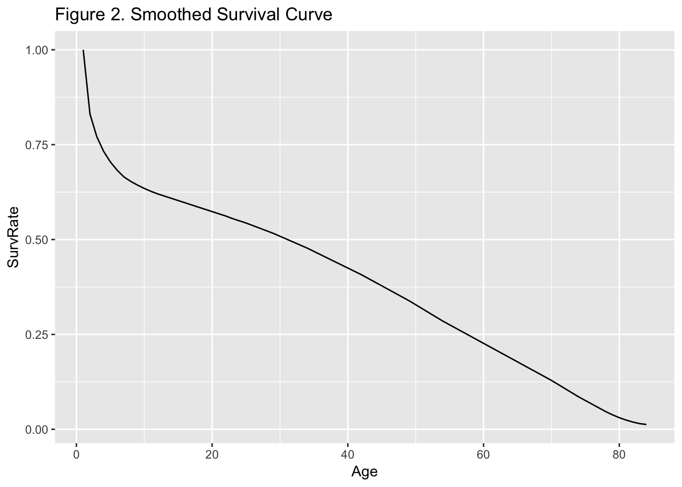
many parts of the world. Plotting a smoothed version of survival
$S$ (Figure 2) shows a sharp drop in survival for
infants, and then an almost constant decline all the way out to age 80
or so (granted, this was in the 1650’s).
x9 <- halley
x9$AtRisk <- x9$Persons
x9$Deceased <- -c(0, diff(x9$AtRisk, 1))
x9$Rate <- 1 - x9$Deceased/x9$AtRisk
x9$SurvRate <- cumprod(x9$Rate)
x9 %>% ggplot() + geom_line(aes(x = Age, y = SurvRate)) +
  ggtitle("Figure 2. Smoothed Survival Curve")
From the same data we can also plot (Figure 3) the mortality or hazard
rate, that is, the instantaneous rate of change in survival, which
shows the classic bathtub-curve shape — a sharp drop in mortality after
birth, then a near constant period corresponding to the prime of life,
with mortality again increasing as old age approaches.
x9 %>% dplyr::filter(Age > 1, Age < 84) %>%
  ggplot() + geom_line(aes(x = Age, y = 1 - Rate), color = "red") -> plot2
plot2 + ylab("Smoothed Mortality Rate") +
  ggtitle("Figure 3. Smoothed Hazard Rate Curve")

Modern survival analysis
The field of survival analysis has come a long ways since these and
other pioneering efforts. With the explosion of mathematical and
statistical theory in the 20th century and the ongoing advances in
computing, we are now able to analyze large quantities of survival and
reliability data and assess what underlying causes of death or failure.
Insurance, manufacturing, medicine, all rely on statistical models of
frailty and survival to inform business decisions, maintenance
schedules, and patient treatment. Survival analysis is a vital and
burgeoning area of research, and new methodologies are continually
emerging.
Using methods analogous to those found in linear regression, we can
assess differences in survival based on different explanatory or
environmental factors. As an example, consider data collected on long
cancer deaths by age and gender:
library(survival)
head(lung)
##   inst time status age sex ph.ecog ph.karno pat.karno meal.cal wt.loss
## 1    3  306      2  74   1       1       90       100     1175      NA
## 2    3  455      2  68   1       0       90        90     1225      15
## 3    3 1010      1  56   1       0       90        90       NA      15
## 4    5  210      2  57   1       1       90        60     1150      11
## 5    1  883      2  60   1       0      100        90       NA       0
## 6   12 1022      1  74   1       1       50        80      513       0
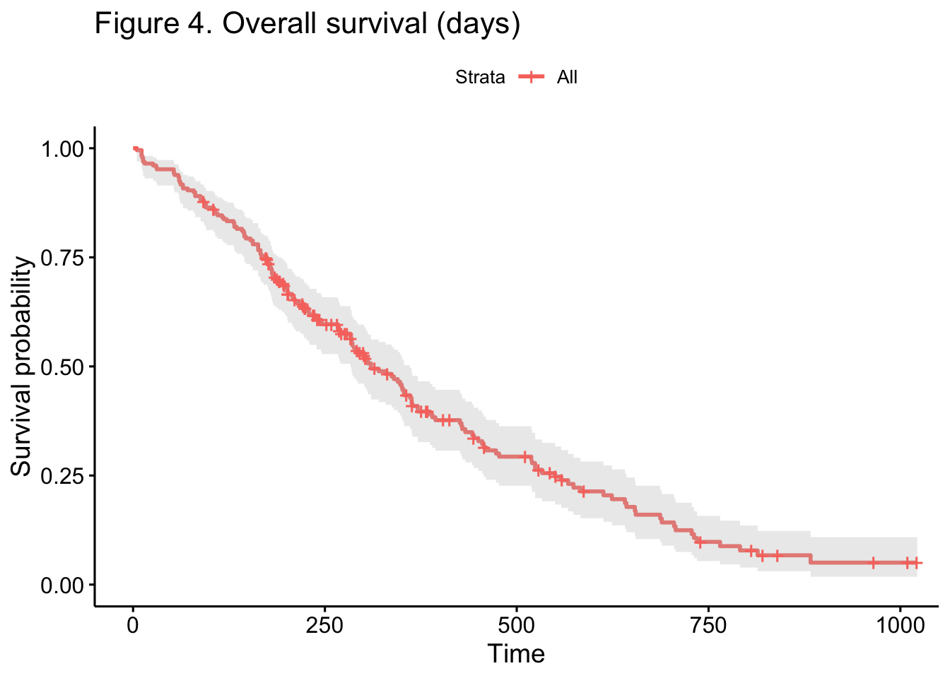
A modern version of a life table estimator, known as the Kaplan-Meier
Estimator, displays the overall survival curve in Figure 4:
lung$SurvObj <- with(lung, Surv(time, status == 2))
lung.S1 <- survfit(SurvObj ~ 1, data = lung, conf.type = "log-log")
ggsurvplot(lung.S1, conf.int = T) + ggtitle("Figure 4. Overall survival (days)")
A natural question is to ask what effect, if any, gender has on the
survival of lung cancer patients. This can be easily determined
graphically (in Figure 5) as well as statistically, showing separate
survival curves for men (red) and women (green).
lung.S2 <- survfit(SurvObj ~ sex, data = lung,
                   conf.type = "log-log")
lung.S2
## Call: survfit(formula = SurvObj ~ sex, data = lung, conf.type = "log-log")
##
##         n events median 0.95LCL 0.95UCL
## sex=1 138    112    270     210     306
## sex=2  90     53    426     345     524
ggsurvplot(lung.S2, conf.int = T) + ggtitle("Figure 5. Survival curves by gender (days)")
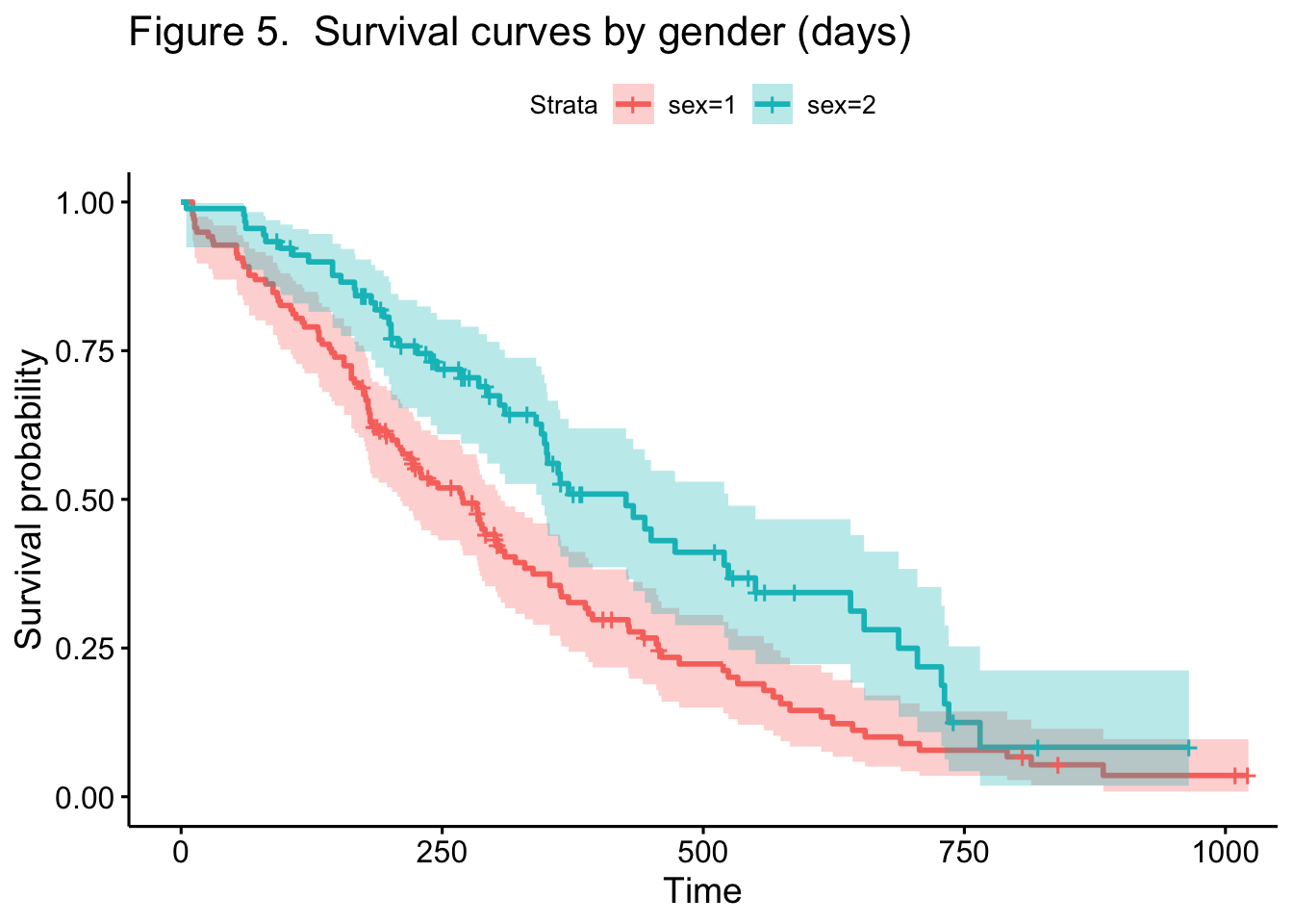
In this case, women have a median survival time of 426 days vs. 270 for
men, and this difference is significant at a 95% level of confidence –
the upper and lower confidence limits for median survival of the two
groups do not overlap.
In closing, this blog post has only scratched the surface of survival
analysis techniques. A list of more sophisticated models for survival
include:
- parametric models (used especially in manufacturing and engineering
reliability studies) - semi-parametric models (such as the Cox Proportional Hazards Model,
which allows for analysis of censored data) - competing risk models
- Bayesian models,
- models with time-varying covariates and parameters
A good place to start for further research is to look at the R package
survival by Therneau. A good general reference for survival analysis
methodology is “Survival Analysis: Techniques for Censored and Truncated
Data” by Klein and Moeschberger.