
In a previous post we gave an introduction to Stan and PyStan using a basic Bayesian logistic regression model. There isn’t generally a compelling reason to use sophisticated Bayesian techniques to build a logistic regression model. This could be easily replicated using simpler techniques. In this post, we shall really unlock the power of Stan and full Bayesian inference in the form of a hierarchical model. Suppose we have a dataset which is stratified into N groups. We have a couple of choices for how to handle this situation. We can effectively ignore the stratification and pool all of the data together and train a model on all of the data at once. The cost of this is that we are losing information added by the stratification. We can fit a separate model for each group, but this runs the risk of overfitting. As we shall see below, groups with few observations will typically represent outliers, but this is not indicative that all observations in the group will behave the same way. If some of the groups have few samples and have significant outlying behavior, it is likely that the behavior is driven by the small sample size rather than the group exhibiting behavior that deviates significantly from the mean behavior.
Hierarchical models split the difference between these two approaches; groups are each assigned their own model coefficients, but, in the Bayesian language, those model coefficients are drawn from the same prior and thus the coefficient posterior distributions are shrunk toward the global mean. This allows for a model which is robust to overfitting but at the same time remains as interpretable as ordinary regression models.
import matplotlib.pyplot as plt
import pystan as stan
import datetime
import pandas as pd
import numpy as np
from sklearn.model_selection import train_test_split
from sklearn.utils import resample
from scipy.stats import bernoulli
import scipy
import itertools
import arviz as az
import pickle
import geopandas as gpd

SEED = 875367
df_raw = pd.read_csv('LoanStats3b.csv.zip', header=1)
/home/ubuntu/anaconda3/lib/python3.6/site-packages/IPython/core/interactiveshell.py:2785: DtypeWarning: Columns (0,47,123,124,125,128,129,130,133) have mixed types. Specify dtype option on import or set low_memory=False.
  interactivity=interactivity, compiler=compiler, result=result)
df_raw.shape
(188183, 137)
The Data
We shall use the same data that we used in our previous post:
‘loan_amnt’: The amount of principle given in the loan
‘int_rate’: The interest rate
‘sub_grade’: A grade assigned to the loan internally by Lending Club
‘annual_inc’: The lendee’s annual income
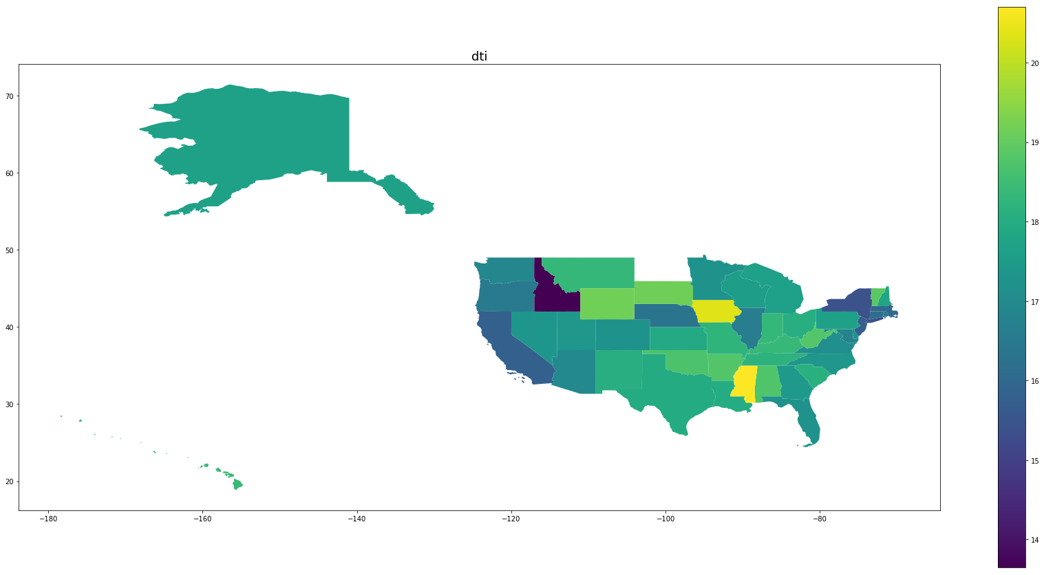
‘dti’: The lendee’s debt-to-income ratio
‘loan_status’: The final status, either “Paid” or “Charged Off”, of the loan
We will also add ‘addr_state’, which is the state in which the borrower lives.
keeps = ['loan_amnt', 'int_rate','sub_grade','annual_inc','dti','addr_state','loan_status']

df = df_raw.loc[:,keeps]

df.loan_status.value_counts()
Fully Paid            148549
Charged Off            28643
Current                10262
Late (31-120 days)       331
In Grace Period          284
Late (16-30 days)         73
Default                   39
Name: loan_status, dtype: int64
def encode_status(x):
    if x == 'Fully Paid':
        return 1
    else:
        return 0
#Slice out loans whose terms haven't expired and numerically encode the final status
df = df[df['loan_status'].isin(["Fully Paid", "Charged Off"])]
df.loan_status = df.loan_status.apply(encode_status)
We encode the sub_grade feature ordinally and treat this as a numerical feature. There are more sophisticated methods we can use on ordinal features, but this will be the topic of a future post.
#Ordinally encode the sub_grade
df.sub_grade = df.sub_grade.apply(lambda x: 5*ord(x[0]) + int(x[1]))
#Strip the label from interest rate
df.int_rate = df.int_rate.apply(lambda x: float(x.split('%')[0]))
features = ['loan_amnt', 'int_rate', 'sub_grade', 'annual_inc', 'dti']
Normalization
We shall use the same normalizations as in the post.
#Transform features to help with normalization.
df['log_int_rate'] = df.int_rate.apply(np.log)
df['log_annual_inc'] = df.annual_inc.apply(np.log)
df['trans_sub_grade'] = df.sub_grade.apply(lambda x: np.exp(x/100))
df['log_loan_amnt'] = df.loan_amnt.apply(np.log)
trans_features = ['log_int_rate', 'log_annual_inc', 'log_loan_amnt', 'trans_sub_grade', 'dti']
df['intercept'] = 1
agg = df[trans_features + ['addr_state']].groupby('addr_state').mean()
num_loans = df[['addr_state', 'intercept']].groupby('addr_state').count()
num_charged_off = df[['addr_state', 'loan_status']].groupby('addr_state').sum()
percentage_charged_off = num_charged_off['loan_status']/num_loans['intercept']
num_loans.intercept.sort_values()
addr_state
IA        1
ID        2
MS        3
NE        3
VT      285
SD      388
WY      421
DE      436
MT      534
AK      535
DC      537
RI      741
NH      828
WV      838
NM      941
HI     1051
AR     1341
UT     1413
OK     1571
KY     1586
KS     1665
TN     1847
SC     1943
IN     2085
LA     2109
WI     2143
AL     2168
OR     2435
NV     2658
CT     2688
MO     2771
MN     3038
CO     3752
MD     4000
AZ     4073
MA     4156
WA     4240
MI     4252
NC     5079
VA     5391
OH     5502
GA     5503
PA     5900
NJ     6751
IL     6836
FL    12197
TX    13673
NY    15365
CA    29517
Name: intercept, dtype: int64
map_df = gpd.read_file('tl_2017_us_state.shx')
INFO:fiona.ogrext:Failed to auto identify EPSG: 7
map_df.shape

map_df.STUSPS.sort_values()
#These states and territories appear in our shape file but not in the data
not_in_data = ['AS', 'GU', 'MP', 'VI', 'PR', 'ND', 'ME']
#Use states as indices to make merging easier
map_df.set_index('STUSPS', inplace=True)

map_df.drop(not_in_data, inplace=True, axis=0)
#This cuts out the Aleutian Islands since they were causing issues rendering the map
map_df.loc['AK', 'geometry'] = map_df.loc['AK', 'geometry'][48]
map_df = pd.concat([map_df, agg], axis=1)
map_df['number_of_loans'] = num_loans['intercept']
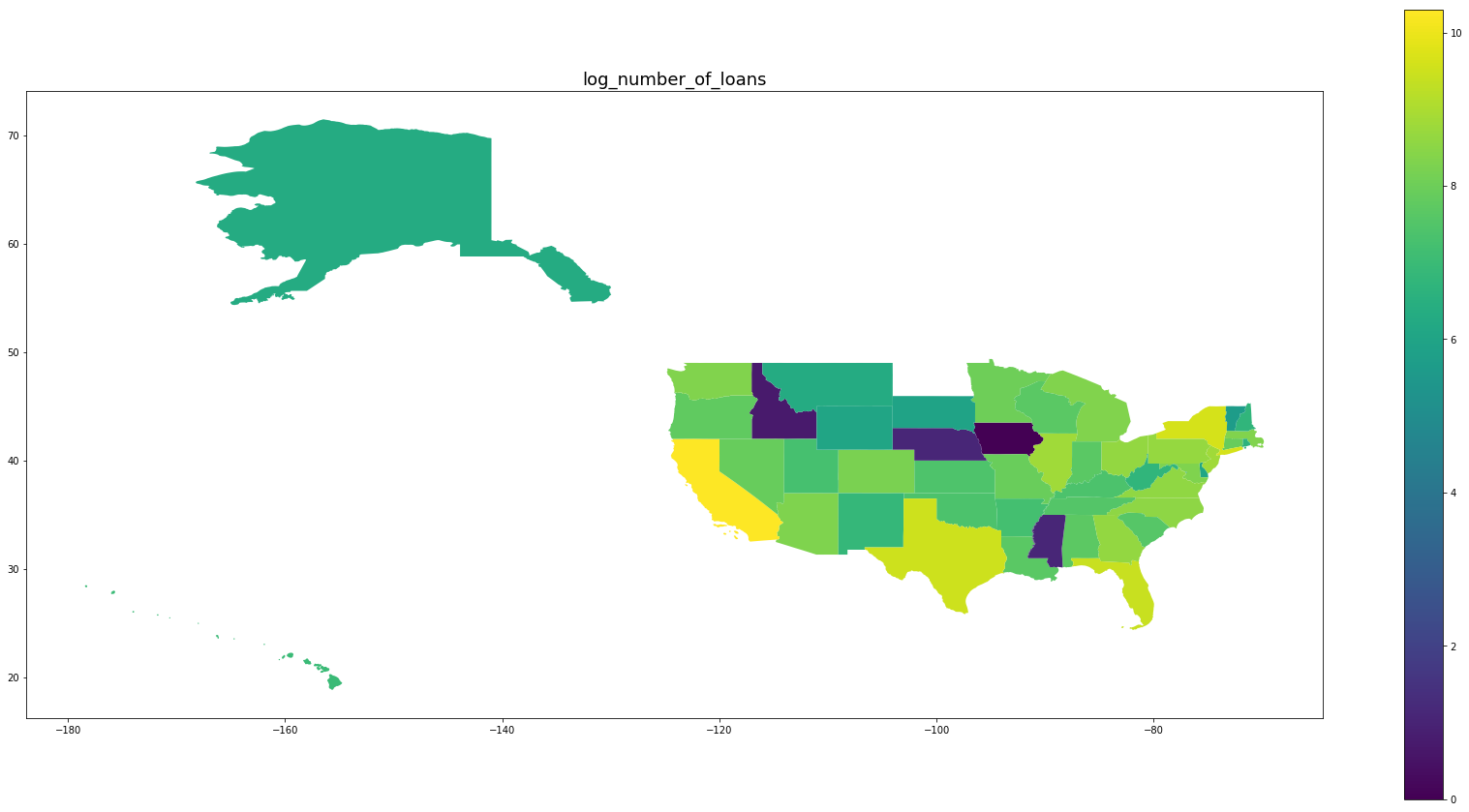
map_df['log_number_of_loans'] = map_df.number_of_loans.apply(np.log)
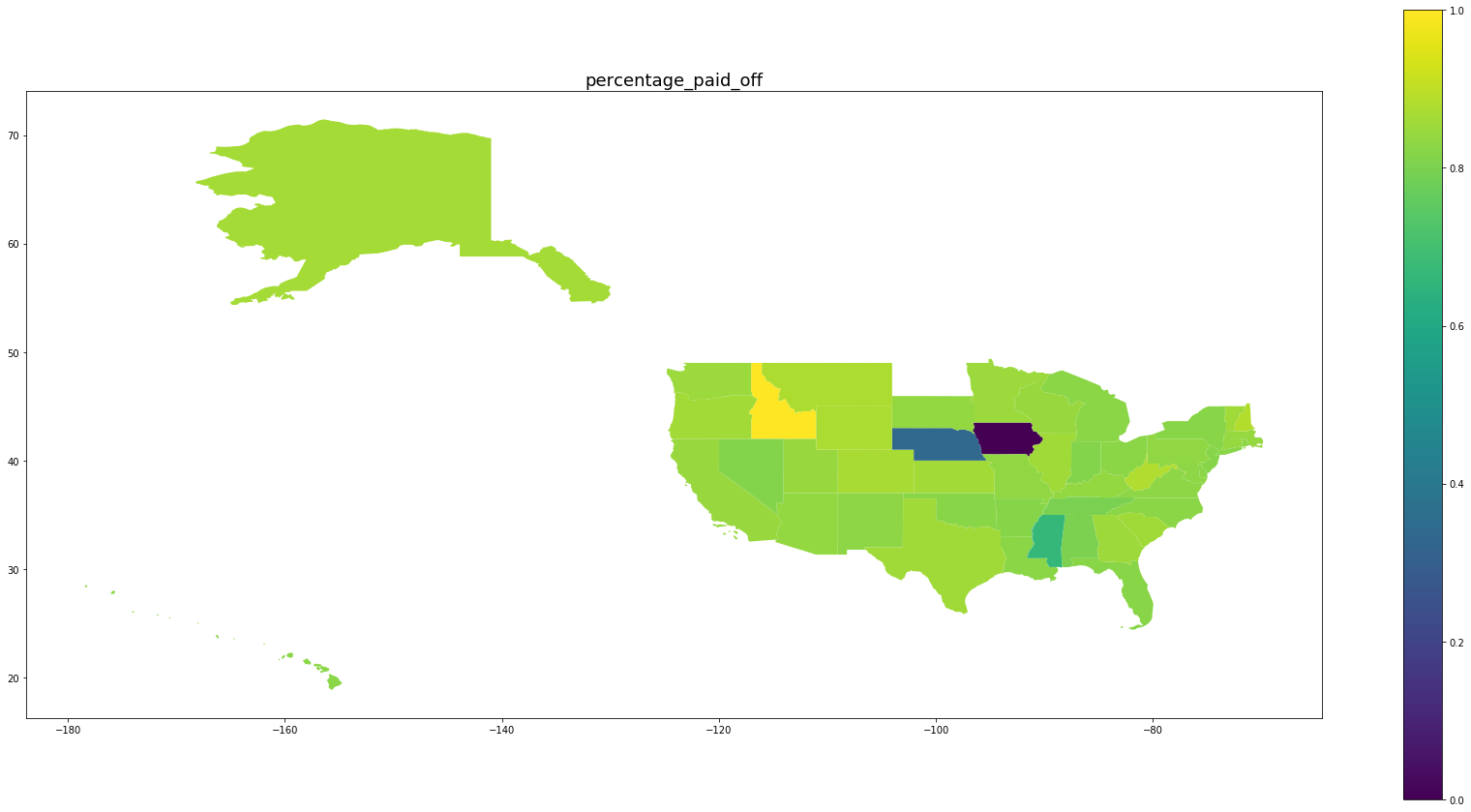
map_df['percentage_paid_off'] = num_charged_off['loan_status']/map_df.number_of_loans
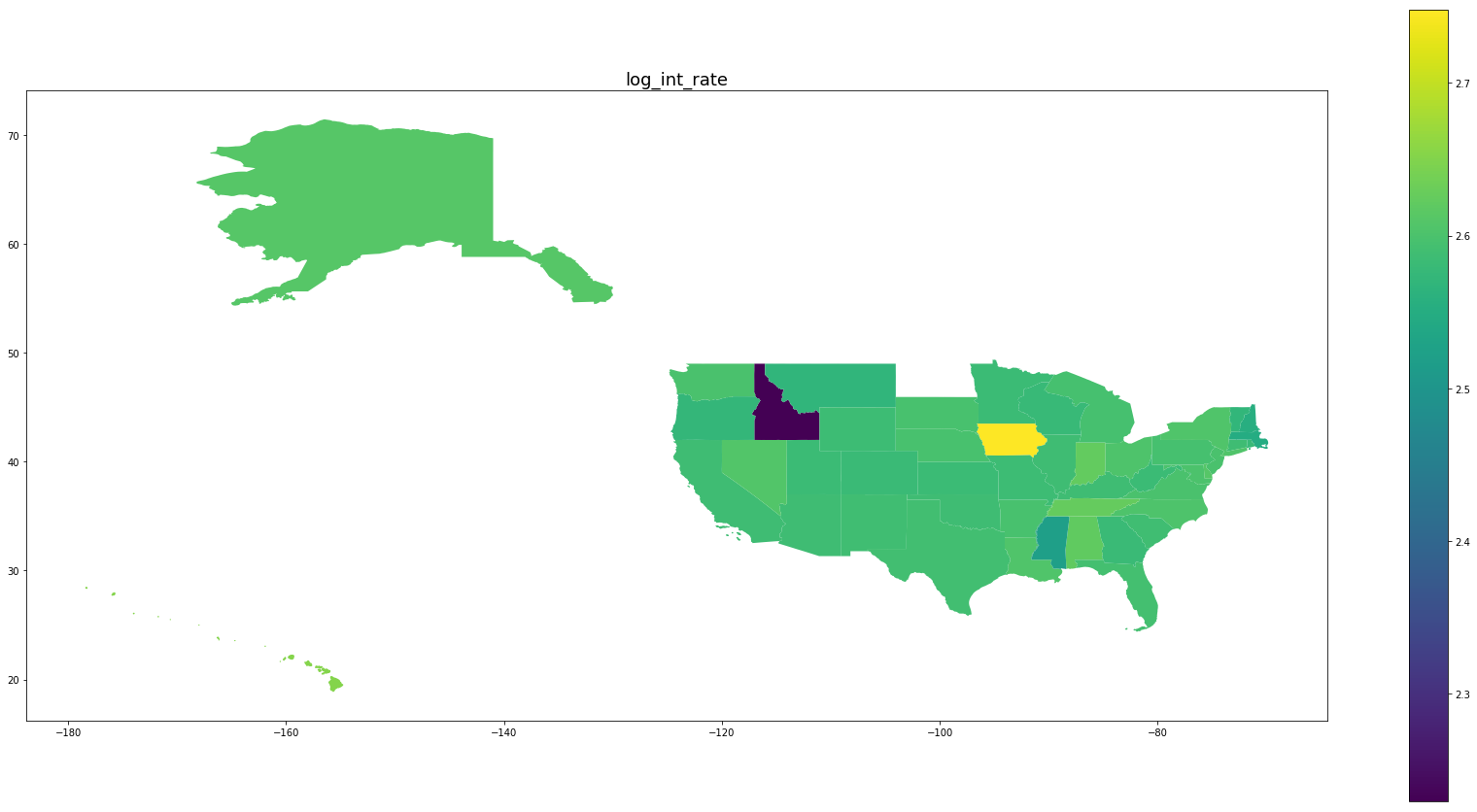
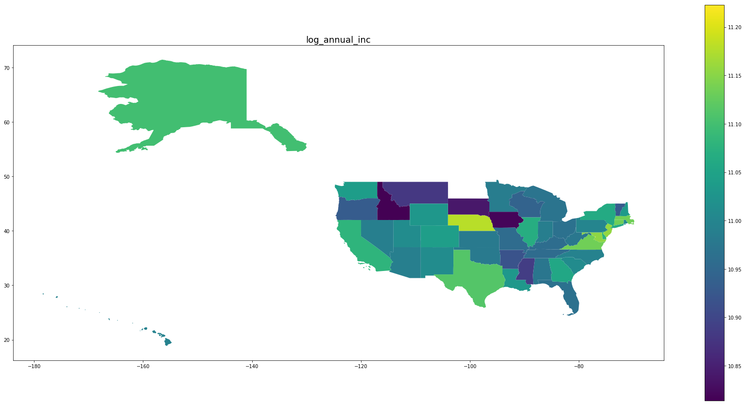
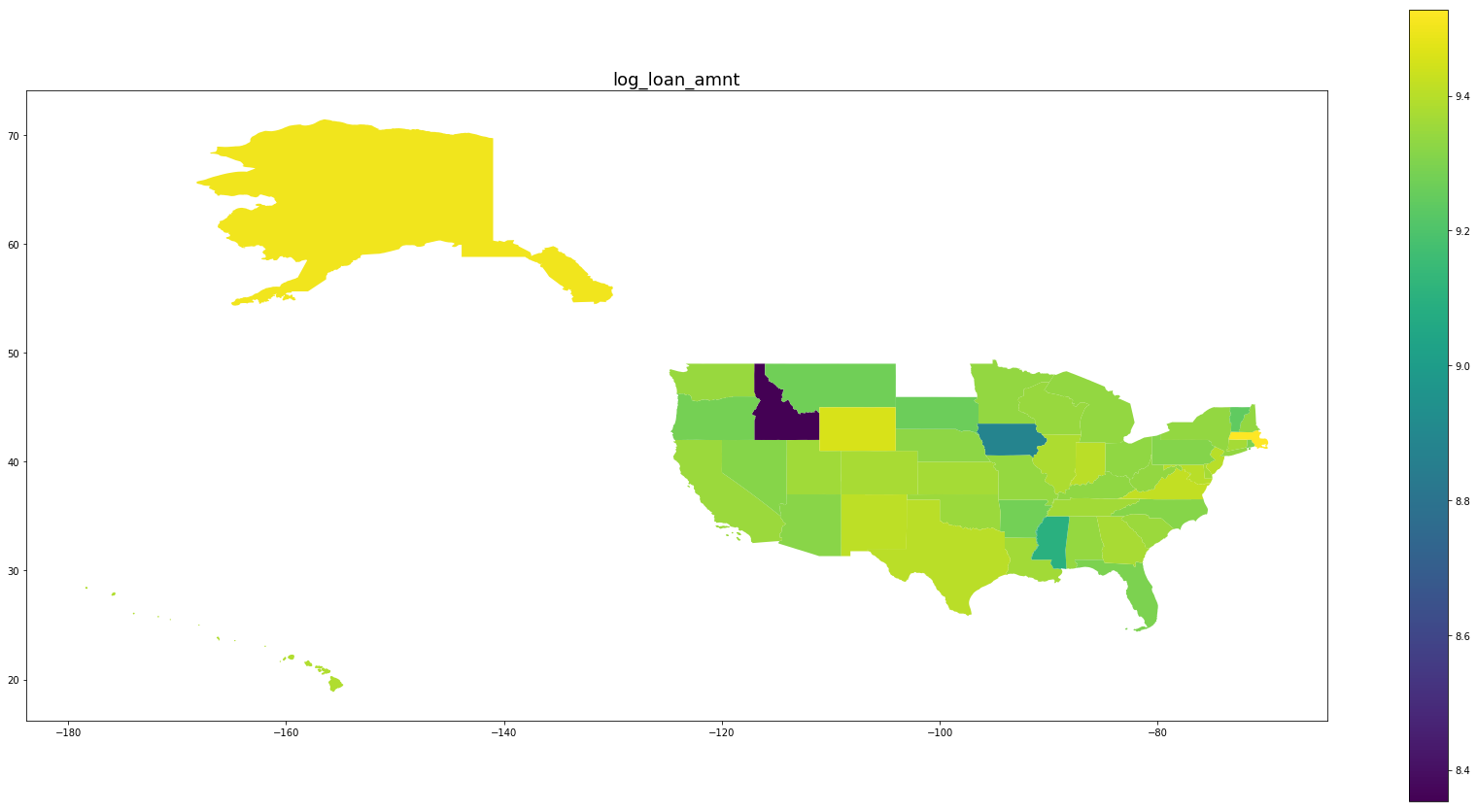
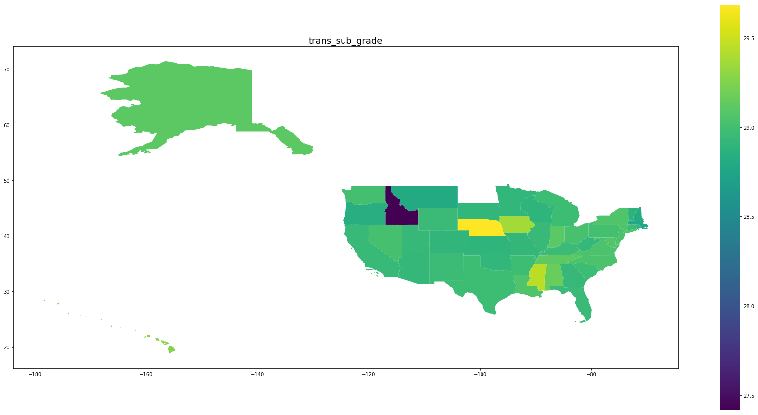
Below we see plots of averages of each feature by state as well the log of the number of observations and a normalized percentage of charged off loans. Notice that the outliers are Idaho, Iowa, Mississippi, and Nebraska, the states with the fewest data points.
for feature in trans_features + ['log_number_of_loans', 'percentage_paid_off']:
    ax = map_df.plot(feature, figsize=(30,15), legend=True)
    ax.set_title(feature, fontsize=18)
final = df.loc[:,trans_features+['addr_state','loan_status']]
final['addr_state_codes'] = final.addr_state.astype('category').cat.codes + 1
final['intercept'] = 1

train, test = train_test_split(final, train_size = 0.8, random_state=SEED)
print(len(train))
print(len(test))
141753
35439
/home/ubuntu/anaconda3/lib/python3.6/site-packages/sklearn/model_selection/_split.py:2026: FutureWarning: From version 0.21, test_size will always complement train_size unless both are specified.
  FutureWarning)
final.head()
| log_int_rate | log_annual_inc | log_loan_amnt | trans_sub_grade | dti | addr_state | loan_status | addr_state_codes | intercept | |
|---|---|---|---|---|---|---|---|---|---|
| 0 | 2.030776 | 12.691580 | 10.239960 | 26.575773 | 18.55 | CA | 1 | 5 | 1 |
| 2 | 2.706716 | 11.407565 | 9.314700 | 29.370771 | 3.73 | NY | 1 | 33 | 1 |
| 3 | 2.604909 | 11.512925 | 10.085809 | 28.502734 | 22.18 | MI | 1 | 22 | 1 |
| 4 | 2.396986 | 10.404263 | 8.987197 | 27.660351 | 15.75 | CO | 0 | 6 | 1 |
| 6 | 2.672078 | 11.492723 | 9.615805 | 29.078527 | 6.15 | NY | 1 | 33 | 1 |
train.addr_state.head()
158925    MI
44469     PA
184000    WA
69645     WV
185689    SC
Name: addr_state, dtype: object
Standard Normalization
Finally, we shall perform some standard normalization of the data in order to improve performance of the sampler.
means = train.loc[:, trans_features].mean()

standard_dev = train.loc[:, trans_features].std()

train.loc[:, trans_features] = (train.loc[:, trans_features] - means)/standard_dev

test.loc[:, trans_features] = (test.loc[:, trans_features] - means)/standard_dev
/home/ubuntu/anaconda3/lib/python3.6/site-packages/pandas/core/indexing.py:537: SettingWithCopyWarning:
A value is trying to be set on a copy of a slice from a DataFrame.
Try using .loc[row_indexer,col_indexer] = value instead

See the caveats in the documentation: http://pandas.pydata.org/pandas-docs/stable/indexing.html#indexing-view-versus-copy
  self.obj[item] = s
The Stan Model
Below there are two Stan models. The first is a simple model based on the model specification given in the introduction. This model suffers from a difficulty in described and visualized excellently in this blog post. The second model is the reparameterization describe in Dr. Wiecki’s post and recoded in Stan. If what is happening here seems contrived and confusing, think back to when you took vector calculus; this reparameterization is akin to changing variables to make an integral computation easier. In more sophisticated mathematical language, we are reparameterizing a particular manifold in order to make an integral computation more efficient.
hierarchical_model = '''
data {
    int<lower=1> D;
    int<lower=0> N;
    int<lower=1> L;
    int<lower=0,upper=1> y[N];
    int<lower=1,upper=L> ll[N];
    row_vector[D] x[N];
}
parameters {
    real mu[D];
    real<lower=0> sigma[D];
    vector[D] beta[L];
}
model {
    mu ~ normal(0, 100);
    for (l in 1:L)
        beta[l] ~ normal(mu, sigma);
    for (n in 1:N)
        y[n] ~ bernoulli(inv_logit(x[n] * beta[ll[n]]));
}
'''
noncentered_model = '''
data {
int N;
int D;
int L;
row_vector[D] x[N];
int<lower=0, upper=L> ll[N];
int<lower=0, upper=1> y[N];
}
parameters {
vector[D] mu;
vector<lower=0>[D] sigma;
vector[D] offset[L];
real eps[L];
}
transformed parameters{
vector[D] theta[L];
for (l in 1:L){
theta[l] = mu + offset[l].*sigma;
}
}
model {
vector[N] x_theta_ll;
mu ~ normal(0,100);
sigma ~ cauchy(0,50);
eps ~ normal(0,1);
for (l in 1:L){
    offset[l] ~ normal(0,1);
}

for (n in 1:N){
y[n] ~ bernoulli_logit(x[n]*theta[ll[n]] + eps[ll[n]]);
}
}
'''
Compiling the Stan model
Stan is a domain-specific language written in C++. The model must be compiled into a C++ program. The upshot of this is that a model can be compiled once and reused as long as the data schema does not change. Here we are serializing the model and then deserializing later to save the compilation step.
sm = stan.StanModel(model_code=noncentered_model, model_name='HLR')
pickle.dump(sm, open('HLR_model_20190522.pkl','wb'))
sm = pickle.load(open('HLR_model_20190522.pkl', 'rb'))
#The sampling methods in PyStan require the data to be input as a Python dictionary whose keys match
#the data block of the Stan code.
data = dict(x = train.loc[:,trans_features].values,
            N = len(train),
            L = len(train.addr_state.value_counts()),
            D = len(trans_features),
            ll = train.addr_state_codes.values,
            y = train.loan_status.values)
Sampling
The sampling step takes about 90 minutes on a compute-optimized AWS EC2 instance. This is another object that can be serialized for later use. It does depend on the Stan model that was used for sampling, and so the model deserialization step above is necessary to deserialize the samples as well. If an hour and a half seems like a long time to sample, bear in mind that we are drawing 6000 samples from 49 states times 6 features, so 6000 samples for almost three hundred model parameters.
fit = sm.sampling(data=data, chains=4, iter=2000, warmup=500)
pickle.dump(fit, open('HLR_fit_20190522.pkl', 'wb'))
fit = pickle.load(open('HLR_fit_20190522.pkl','rb'))
/home/ubuntu/anaconda3/lib/python3.6/site-packages/pystan/misc.py:399: FutureWarning: Conversion of the second argument of issubdtype from `float` to `np.floating` is deprecated. In future, it will be treated as `np.float64 == np.dtype(float).type`.
  elif np.issubdtype(np.asarray(v).dtype, float):
#We suppress the output from this print statement because it is large, but this give a lot of useful information about
#the posteriors
print(fit)
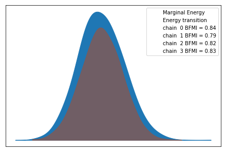
Assessment of Convergence
We use the Arviz library again to give a brief assessment of convergence of the MCMC method. Refer back to the previous post for an interpretation of the metrics below. We seem to be in good shape.
inf_data = az.convert_to_inference_data(fit)
az.plot_energy(inf_data)
<matplotlib.axes._subplots.AxesSubplot at 0x7f8a3b3dae10>
az.rhat(inf_data).max()
<xarray.Dataset>
Dimensions:  ()
Data variables:
    mu       float64 1.0
    sigma    float64 1.0
    offset   float64 1.0
    eps      float64 1.0
    theta    float64 1.0
Prediction
If you have read the first post in this series, you may have noticed that we are using an unbalanced training set. Our approach to prediction is going to be slightly different in this post. Our approach here will be to use random number generation and the posteriors generated by the MCMC to generate synthetic outcomes for each sample. Notice the similarity of our scoring code to the Stan model definition above.
#This dictionary allows us to move from 3-tensors to a dictionary of 2-tensors for each state.
state_translate = dict(list(zip(train.addr_state_codes.unique()-1, train.addr_state.unique())))
#Extracts the samples from the fit object.
samples = fit.extract()
theta = samples['theta']
theta.shape
(6000, 49, 5)
theta_state = {}
for j in range(49):
    theta_state[state_translate[j]] = theta[:,j,:]
theta_state['AK'].shape
(6000, 5)
eps = samples['eps']
eps_state = {}
for j in range(49):
    eps_state[state_translate[j]] = eps[:,j]
#Here we are using the same "model" as in the Stan code above to generate so-called synthetic outcomes for each
#sample in our posterior. E.g. each sample is randomly assigned an outcome according to
#y ~ bernoulli(inv_logit(x.theta + eps))
outcomes = {}
for j in range(49):
    s = state_translate[j]
    vals = test.loc[test.addr_state==s].loc[:,trans_features].values
    outcomes[s] = np.dot(theta_state[s], np.transpose(vals)) + np.repeat(eps_state[s].reshape(-1,1), vals.shape[0], axis=1)
    outcomes[s] = scipy.special.expit(outcomes[s])
    outcomes[s] = bernoulli.rvs(p=outcomes[s], size=outcomes[s].shape, random_state=SEED)
means = {}
for j in range(49):
    means[state_translate[j]] = outcomes[state_translate[j]].sum(axis=0).mean()/6000
/home/ubuntu/anaconda3/lib/python3.6/site-packages/ipykernel_launcher.py:3: RuntimeWarning: Mean of empty slice.
  This is separate from the ipykernel package so we can avoid doing imports until
/home/ubuntu/anaconda3/lib/python3.6/site-packages/numpy/core/_methods.py:85: RuntimeWarning: invalid value encountered in double_scalars
  ret = ret.dtype.type(ret / rcount)
map_df['predicted_percentage_paid_off'] = pd.DataFrame.from_dict(means, orient='index')
#Notice the similarity in outcomes for each column
map_df.loc[:, ['predicted_percentage_paid_off','percentage_paid_off']]
| predicted_percentage_paid_off | percentage_paid_off | |
|---|---|---|
| AK | 0.860305 | 0.863551 |
| AL | 0.810346 | 0.803506 |
| AR | 0.819547 | 0.818792 |
| AZ | 0.831808 | 0.837957 |
| CA | 0.848516 | 0.847003 |
| CO | 0.873511 | 0.870203 |
| CT | 0.839806 | 0.840402 |
| DC | 0.899450 | 0.901304 |
| DE | 0.835026 | 0.827982 |
| FL | 0.823190 | 0.820940 |
| GA | 0.849306 | 0.852081 |
| HI | 0.816192 | 0.824929 |
| IA | NaN | 0.000000 |
| ID | NaN | 1.000000 |
| IL | 0.860913 | 0.856349 |
| IN | 0.806308 | 0.814388 |
| KS | 0.858311 | 0.860661 |
| KY | 0.835005 | 0.837957 |
| LA | 0.828594 | 0.824561 |
| MA | 0.841324 | 0.842156 |
| MD | 0.837103 | 0.831000 |
| MI | 0.830536 | 0.825729 |
| MN | 0.851228 | 0.850560 |
| MO | 0.838572 | 0.834356 |
| MS | NaN | 0.666667 |
| MT | 0.874037 | 0.878277 |
| NC | 0.831902 | 0.826147 |
| NE | 0.519417 | 0.333333 |
| NH | 0.885235 | 0.885266 |
| NJ | 0.817354 | 0.818694 |
| NM | 0.828945 | 0.829968 |
| NV | 0.816005 | 0.812641 |
| NY | 0.824079 | 0.823690 |
| OH | 0.830508 | 0.827336 |
| OK | 0.825519 | 0.820496 |
| OR | 0.856078 | 0.860780 |
| PA | 0.832139 | 0.834407 |
| RI | 0.845055 | 0.828610 |
| SC | 0.858934 | 0.858466 |
| SD | 0.844788 | 0.837629 |
| TN | 0.801999 | 0.799675 |
| TX | 0.855880 | 0.856286 |
| UT | 0.847335 | 0.845718 |
| VA | 0.822405 | 0.830458 |
| VT | 0.848991 | 0.856140 |
| WA | 0.850302 | 0.849528 |
| WI | 0.856926 | 0.844144 |
| WV | 0.867103 | 0.879475 |
| WY | 0.874102 | 0.874109 |
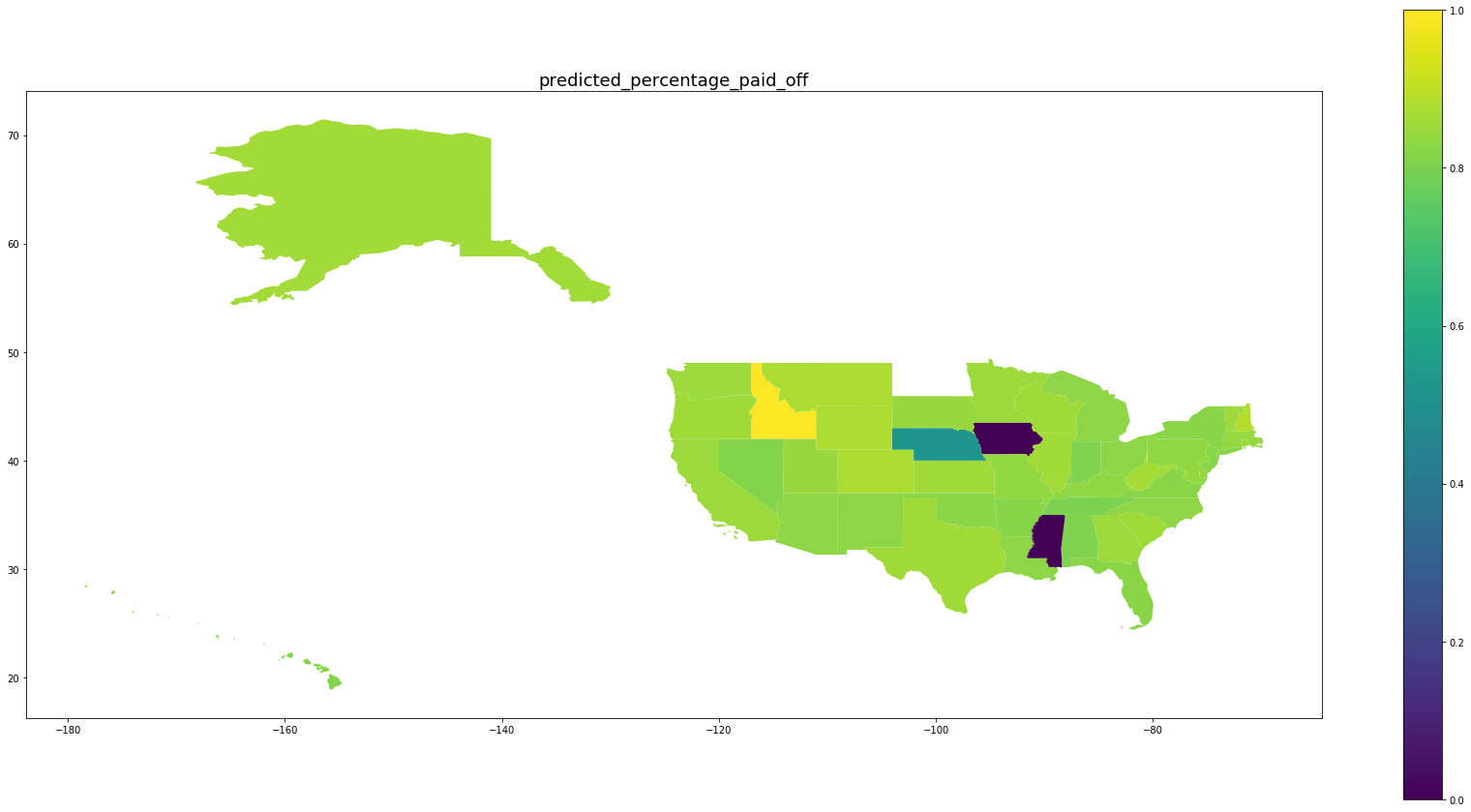
#MS, IA, and ID did not appear in the test set. These choices will help keep the color schemes consistent in the
#chloropleths.
map_df.loc[['MS','IA'],'predicted_percentage_paid_off'] = 0.0

map_df.loc[['ID'],'predicted_percentage_paid_off'] = 1.0
Be wary of the scales on the right. We see that for states with large numbers of oberservations, the percentage of predicted paid off loans matches the percentage of paid off loans in that state while for states with fewer observations, the behavior is drawn back toward the mean.
for per in ['predicted_percentage_paid_off', 'percentage_paid_off']:
    ax = map_df.plot(per, figsize=(30,15), legend=True)
    ax.set_title(per, fontsize=18)

Concluding Remarks
The model we have presented represents an elegant way to handle stratified data in a way that is robust to overfitting but remains highly interpretable. There are few methods that can achieve this balance! In our scoring method, we are able to generate predictions in line with probability distributions in the training data. In order to make loan-level predictions, we simply choose a probability threshold which is acceptable for our use-case, and make a prediction based on the probability of default being above or below that threshold.